


AI is increasingly playing a role in areas where its decisions can have real-world impacts. Banks rely on models to detect fraud. Manufacturers rely on these models to save energy, catch machine issues early, and help operators make smarter choices. However, turning a model from a data scientist’s notebook into a trusted tool for industry is a big leap that requires a lot of work.
We understand that diagnosing the problem isn’t always straightforward. When an AI system encounters issues in production, the usual instinct is to enhance the model by increasing accuracy, retraining it, gathering more data, or trying a different model. These efforts are valuable, but they address only one part of the puzzle. Sometimes, even a highly accurate model can be challenging to deploy, risky to update, sensitive to the specific context, or difficult to revert. At that stage, the real challenge often lies not in the model itself, but in the overall architecture.
Classical software architectures and their design principles evolved in a world where logic was mostly deterministic and relatively static, changing gradually through software releases. In contrast, AI disrupts all three premises. The behavior of a model does not depend on any specific lines of code. Its reliability may vary with different inputs, depending on how the model interprets them. The same software version can behave differently at different times, even without code changes.
In this article, we believe that production AI architecture mainly focuses on managing that volatility. It’s about deciding which types of change are okay to spread through the system and where to set boundaries to stop them. That is the reason we focus on five patterns. Please note that these patterns are not meant to be an exhaustive list of all the requirements for AI production. Instead, each pattern highlights a specific type of change that AI brings about or emphasizes, based on architectural ideas that existed even before modern AI technologies. This approach helps us understand the core influences of AI in a clear and approachable way.
Training–Serving Separation improves the entire model lifecycle by letting models be retrained on fresh data independently, without changing the surrounding application. Hexagonal Architecture considers different deployment environments. Factors like cameras, protocols, plant IT, site topology, PLCs, and integration surfaces may vary from one installation to another, even when the core domain problem stays the same. The Training–Inference Pipeline Segregation highlights key differences in how workloads behave. Learning naturally needs more resources and happens in a more relaxed, asynchronous way, whereas inference is usually delay-sensitive and critical in production settings. By keeping these tasks separated, we can avoid any unnecessary conflicts and ensure smoother operation. Simplex Architecture addresses a different boundary – the boundary of trust and authority. A probabilistic model may be useful, but it shouldn’t be allowed to make every decision on its own. Runtime confidence, operating conditions, and deterministic constraints can determine when control must shift to a safer path.
Finally, an Inference Gateway really comes into play when a single model expands into a whole fleet. Now, models have versions, rollout statuses, hardware locations, shadow deployments, and various routing rules. At this stage, choosing the right model becomes an important part of the overall architecture. The order in which you manage models matters. Routing traffic across multiple models doesn’t make much sense until you see each model as a versioned, production-quality artifact rather than just a file tucked inside an application. Similarly, separating authority from an AI model with a Simplex-style approach only makes sense after establishing domain constraints and safety protocols externally. As the AI system grows, its structure naturally evolves. Solving one boundary often uncovers the next exciting challenge to explore.
It is also essential to consider what we leave out. Characteristics such as feature stores, drift detection, data versioning, labeling, and more are vital for production AI. They show us what the system needs to do. In contrast, the five patterns presented in this paper address a different problem: how do we break up the system to prevent a single change from disrupting everything else?
We should also distinguish patterns across specific model families. Although RAG systems for large language models are useful, they may lose relevance if the model family changes. The patterns described in this article can be used irrespective of changes in model families.
For each pattern, we’ll explore how it works, its advantages and disadvantages, and, just as importantly, when it might not be suitable. To make these architectural choices clear, we’ll stick to a single system throughout this article. Think of it as a car factory with three production lines, each welding about 40–60 body panels per hour. A computer-vision model watches the welds in real time, sorting each panel as acceptable, requiring rework, or scrap. Ultimately, this classification guides the panel through the next steps in the production process.
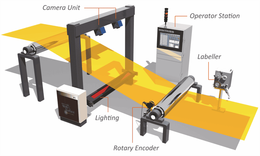
Picture 1: Industrial computer vision defect detection system
This is when a seemingly trivial classification problem becomes an operational one. An incorrect prediction can lead to rejecting a good panel, accepting a faulty panel for further processing, or an unnecessary line stop. In our case, a line stop is communicated to the Programmable Logic Controller (PLC) and costs about €2,400 per minute.
This system has been running for eighteen months and includes three trained models, each designed to account for the lighting, weld-gun calibration, and panel geometry for that production line.
Now, a new weld gun was introduced on Line A, the seam profile changed, and the fourth model is being evaluated. At first glance, the task seems clear – train and deploy a new model.
But this is exactly when architectural questions come into play. Which should be deployed – a new model or a new application? Do we keep the previous model for rollback? Do we update the integration logic for Line A with the model as well? What would happen if the new model reacts differently to production traffic? And the first pattern we consider is precisely designed for this boundary.
Training-Serving Separation
The first challenge we need to address with a new architectural approach is how to frequently update AI/ML models in production without breaking the systems that rely on them. The trick is that AI introduces a new kind of volatility, and the logic changes not because developers wrote new code, but because data shifts.
However, in early deployments, training code (used to train the model) and serving code (used to run the model in production) are often intertwined. A new model release means redeploying the entire application. If that model performs worse in real-world conditions or fails due to new data it hasn’t seen before, the Ops team rushes to roll it back and hopes nothing else is affected. However, with this tight coupling, the lack of versioning, and the absence of logging, updates and rollbacks become painful, unmanageable, and even unpredictable.
This coupling creates a fundamental contradiction: models must change frequently to remain accurate, while production systems must change rarely to remain reliable.
This is precisely where the first and most fundamental architectural pattern for production AI can save us. Training-Serving Separation splits the AI system into three layers that can be deployed independently. This prevents model changes from forcing full system redeployments and prevents business rules from leaking into model code.
First comes the model layer. This is a trained AI/ML model artifact (ONNX, TFLite, Pickle file, etc.) considered as a versioned release. It has an ID, a well-defined input schema, and a recorded evaluation benchmark. Deploy it in a model registry and load it from there. Don’t embed it directly in the application code.
The second is the serving layer. This is a stateless, thin runtime service that loads a model artifact and provides inference via API. It should handle batching, hardware acceleration, and latency targets. Do not place any business rules here.
And third is the business view layer. This is where the system translates predictions into actions/messages relevant to the business domain. Here features (variables describing characteristics of observations for a machine learning model) are prepared, thresholds are applied, output is validated, and results are formatted for further consumption. This is where a score of 0.87 turns into “flag for manual review”
We should explicitly address three failure cases. If the registry is unavailable during inference, the serving layer should keep operating using the most recent valid copy of the artifact and issue a health warning. However, it must not accept requests without a model or with an unknown model, as this would be worse than operating in a degraded mode. If the input structure changes (such as renaming, removing, or changing data types), the model will still provide high-confidence predictions, even for inputs that may now mean something different than they did during training. This problem can be addressed only by validating each inference request against the registered schema during runtime. In addition, the serving layer must detect a corrupt artifact upon loading, not upon registration: it should verify the artifact’s on-disk checksum against the registered hash each time the serving layer starts.
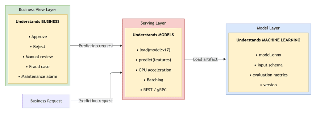
Picture 2: Training-Serving Separation
Still, it’s essential to keep in mind the significant trade-offs involved in this case. Firstly, separation turns the deployment problem into a dependency problem. The registry becomes a runtime dependency with its own availability budget. It means that you have two versioning schemes instead of one (the artifact and the schema contract), and they must be coupled. Otherwise, you will silently validate against the wrong things. Moreover, the serialization step and process boundary become part of the inference path, incurring single-digit-millisecond costs per call. Finally, the business view layer is populated with threshold definitions, override logic, formatting, and audit logic, making it the god object you wanted to avoid in the other two layers.
If the application updates more frequently than the model, you get inverted separation overhead because you are spending effort on the registry and contract to shield yourself from volatility that doesn’t exist. For example, an embedded application without proper network connectivity makes using the registry for deployment an anti-pattern, not the default. Likewise, in a pilot scenario where the model is the product, and there is no downstream business logic to protect, three deployments for three developers are redundant.
Hexagonal Architecture for AI Domain Isolation
Even perfect model version control does nothing to help the rest of the system. The inspection software receives video feeds from cameras via proprietary protocols, sends decision outputs to MES/ERP systems, communicates with PLCs that do not accept unexpected input, and applies custom quality-control logic for a particular plant. If such complexity creeps into the serving layer or even into the model itself, the end result will be a system that works solely on one specific production line within a particular plant.
In hexagonal architecture, we put the business logic and safety logic right in the middle and push everything else to the sides. The domain core understands what a prediction means – how to interpret output scores, which thresholds to use, what alarm to raise, and what to tell the operator. It knows nothing about protocols, databases, and transport. All external connections go through adapters, and the core defines their interfaces.
In our case, the core is QualityDecisionService. It receives raw class scores, compares them against the per-SKU production threshold (0.80 for a door inner left), checks whether a critical defects flag overrides the regular flow, and produces the decision to accept, rework, or scrap the part. The camera protocol, MES integration, and PLC triggering are encapsulated as adapters, so the quality engineer who defines the threshold policy is unaffected by the details.
The calls into the core could use ports such as SubmitSensorReading and RequestPrediction. Calls from the core to external capabilities can go through interfaces such as ModelInferencePort, AuditLogPort, or AlarmDispatchPort. The site-specific implementations will show up as adapters such as OpcUaAdapter, KafkaAdapter, or MesRestAdapter. In such a case, any protocol change should add a new adapter, not modify the domain logic. However, this guarantee becomes less useful if the core does not explicitly declare failure behavior and leaves it as an implementation detail of the adapter.
Adapters have timeouts, so those timeouts are part of the port contract in the core: if the inference adapter fails to complete in time, the core returns a fallback decision and moves forward instead of blocking on a possibly never-ending call. Adapters sometimes send corrupted data, so all boundary ports carry explicit schemas (Pydantic or Protobuf) and reject bad messages early instead of passing them into the system, where they could cause harder-to-diagnose errors.
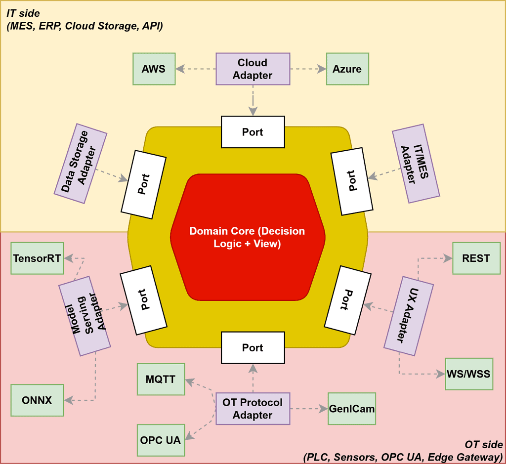
Picture 3: Hexagonal architecture.
When considering how hexagonal architecture is used in AI applications, keep in mind that the system core stays “thin.” Remove the protocols and the persistence, and what is left is usually threshold policy, overriding rules, and output formatting – a few hundred lines. Building an entire port and adapter structure around this will likely yield more scaffolding than domain. The abstraction itself carries a debugging cost. A stack trace spanning three interfaces is longer than one without them – furthermore, teams unfamiliar with this design pattern often introduce transport semantics into port signatures, creating “leaky ports” that provide isolation only in terms of file count, not in practice.
We also need to honestly recognize one important point. Hexagonal architecture helps protect the core domain from external influences. However, it doesn’t shield the model from the domain itself. The model has already learned certain assumptions about the environment from the training data—like lighting conditions, welder calibrations, and panel shapes. Even though the core is protected, that doesn’t mean the model transfers easily. If you take the model to the fourth line, the architecture stays the same, but the predictions might be less dependable.
Training-Inference Pipeline Segregation
When we discuss AI in production, it typically focuses on the model, including its speed and accuracy, as well as the frequency at which it should be retrained. But under the hood, we have two separate types of activities, each with totally different priorities and learning objectives. On the one hand, we have training, where data collection and transformation, training new models, and other difficult, resource-intensive tasks make the model smarter over time.
On the other hand, we have inference – the real-time decision-making layer. This part must respond quickly and constantly. There is no time to wait when a prediction is needed.
Problems start when these two processes share the same infrastructure. Retraining might consume all available resources, slowing inference. Data scientists might push updates that destabilize the real-time system. As a result, the platform becomes too slow for operators and too fragile for engineers to improve.
The solution is to split the training and inference into two separate pipelines. This lets us scale them independently and keep their data paths separate, avoiding competition. This follows the same idea as separating write-heavy work from read-heavy work. But here, it applies to machine learning, not to transactional databases.
The training pipeline involves a high volume of write operations. It ingests raw sensor data and operator feedback, runs feature engineering, triggers retraining, and publishes validated model artifacts to the registry. It runs asynchronously. It should tolerate failures, use queues, and retry when needed.
The inference pipeline is read-heavy. It reads from a prepared feature store, loads a model artifact from the registry, and returns low-latency predictions. Protect it with strict resource limits so training cannot steal CPU, memory, or I/O.
The feedback loop connects the two. Operator corrections and anomaly flags flow back into training as labeled data. Send them asynchronously so inference never blocks feedback.
This split matters most when scale and team structure make interference likely. Use it when inference runs at high frequency, for example, more than a thousand requests per second, and you retrain often, daily or more. In that setup, training and inference will compete for CPU, GPU, and data stores if you keep their logic together. Separation keeps inference stable while training does its heavy work in the background.
This split really makes less sense when inference isn’t used very often, like in a weekly batch-scoring job. In those situations, shared infrastructure usually works well because there’s no urgent need for low latency, and workloads don’t often interfere with each other.
Team structure also matters. Use separation when ML engineering and platform teams work on different schedules. Model updates might occur frequently, while platform changes require stricter change control. Separate pipelines let each team ship at its own pace without breaking the other. But avoid full segregation when a single small team owns everything end to end. While extra services, quotas, and monitoring do introduce some overhead, it’s important to keep in mind that if your team is still working quickly and the system remains small, this additional overhead might actually slow down your progress rather than support it. Finding the right balance can help ensure your team stays agile and effective.
For example, a predictive maintenance system retrains nightly with data from the past 30 days. The training pipeline handles the complex tasks, constructing features and storing them as materialized views in a feature store, such as rolling averages and other pre-calculated statistics.
The inference pipeline remains efficient by solely accessing materialized views, avoiding raw sensor streams, which helps maintain consistent and predictable latency. We have separated learning from doing, but we still face one fundamental challenge. Even with reliable prediction and clear architectural separation, AI still stays probabilistic. It can be exact, but not infallible. In a mission-critical environment, even a minor mistake or misclassification can lead to downtime, defects, or safety incidents. This is where the next pattern comes into play.
Simplex Architecture — Safety-Critical Fallback
Long before AI emerged, industrial automation was already grappling with some of the toughest safety challenges. One of the most trusted solutions from that world is Simplex Architecture design built for situations where making the wrong decision is far more dangerous than missing an optimization.
The main idea is simple: trust an intelligent controller, like an AI model, to manage things when everything’s running smoothly. But when things get uncertain, it’s wise to switch control back to a more reliable, straightforward system. This way, the AI can offer the best suggestion, while a dependable controller helps avoid worst-case outcomes.
The pattern typically relies on three key components working in tandem. The first one is the Advanced Controller, where the AI lives. It is smart and flexible and can boost performance, but by nature it is probabilistic, meaning it’s never 100% certain.
The next is the Baseline Controller. It is slower and less flexible, but it operates on strict, rule-based logic that has been thoroughly tested and designed to provide safe behavior under defined operating conditions. This is the system you can rely on when things go awry.
The Decisions Monitor monitors both. It is a watchdog that constantly checks if the AI is still staying within the rule’s boundaries (e.g., if the AI is confident enough that the model is behaving as expected)
If anything appears incorrect, such as a corrupted sensor reading, a sudden drop in confidence, or delayed inference, the monitor does not wait. It immediately reverses control to the Baseline without disrupting operations. Once everything stabilizes, control can shift back to the AI—usually gradually, and only if safety checks are passed.
There are a few practical ways to bring Simplex Architecture to life. It really depends on where decisions need to be made and how quickly you require a safety fallback.
In many industrial setups, AI and control logic are deployed directly at the edge. In this case, we typically run an AI model on a local GPU or NPU to generate fast, high-quality predictions. Meanwhile, the real-time, deterministic equipment continues to monitor, with hard, deterministic guardrails in place.
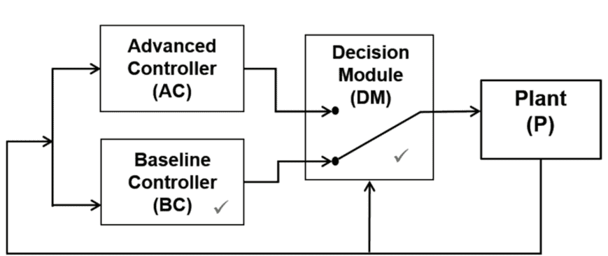
Picture 4: Simplex architecture pattern
Since everything is happening on the device, the Decision Monitor can step in very quickly when needed. This kind of rapid response is crucial when dealing with real machinery and real safety risks.
In other environments, those guardrails reside upstream, in an inference gateway. Here, we have policies and circuit breakers acting as bouncers at the door. If a model starts responding too slowly, confidence drops, or the inputs do not match expectations (i.e., drift), the gateway instantly routes control back to the safe, verified baseline. This setup works well when multiple models or services collaborate to make decisions together.
And sometimes, the safest move is to bring a human into the loop. In this case, the system might pause when the AI shows uncertainty and asks a human to confirm or override the recommendation.
However, no matter how it is built, the principle remains the same: the safe controller is always ready to take over. That way, AI can boost performance when it can—but never at the expense of safety or stability.
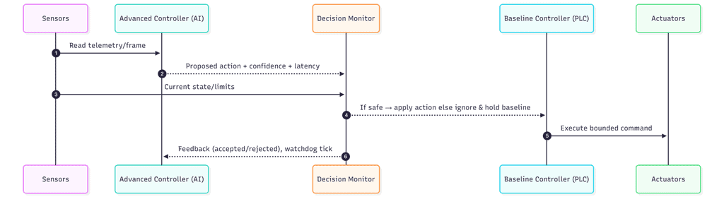
Picture 5: Sequence diagram of how the Simplex method works
A key consideration with this pattern is that the baseline controller tends to be expensive and often underestimated. It needs to be developed, tested, and maintained, but it rarely operates—so it quietly degrades. When it’s finally called into action, it may no longer align with the current process. Additionally, it establishes a performance cap, ensuring that the AI’s output doesn’t exceed the reliable capabilities of the baseline. This means that any measurable improvements will depend on the fallback system you choose to put in place.
Let’s revisit our main goal—once we ensure safety and stability, we’ll unlock one of AI’s greatest benefits in production: the power of multiple models working together. Such systems can adapt on the fly to new materials, new defect types, new operating conditions, and even shifting business priorities without sacrificing reliability.
As our AI solution matures, we naturally move away from the old mindset with one model per problem. Instead, we start deploying multiple models, each performing specialized tasks across edge devices, gateways, and cloud infrastructure. Some are fine-tuned for specific product lines or lighting conditions – others are trained to identify entirely new defects or patterns as they emerge.
As the ecosystem grows, architecture should evolve as well. We need scalable ways to route inference requests, safely test new model versions, and balance traffic across all those moving parts—without introducing chaos or bottlenecks. That is where the next wave of architectural patterns comes in.
Inference Gateway — Controlled Routing at Scale
Instead of exposing every model as an isolated endpoint, modern AI systems introduce an inference gateway or model mesh layer. This layer provides intelligent routing: selecting the right model for each request, balancing loads, running shadow deployments, enforcing guardrails, and collecting unified observations across all inference activity. Inference gateways and a model mesh can help production AI scale without operational complexity growing as intelligence does.
Behind the gateway sits the model mesh, a distributed layer that manages the lifecycle of all deployed models. It treats models as on-demand resources — loading them when needed, unloading them when idle, and automatically allocating them across available hardware.
This design solves a crucial resource problem: most models are not in use 100% of the time. The mesh ensures GPUs, CPUs, and NPUs are used efficiently across hundreds of models, reducing costs without compromising performance. It can prewarm models expected to receive traffic, balance requests across compute nodes, and continuously monitor health. The result is a dynamic, self-managing infrastructure that grows in tandem with your AI ambitions, rather than constraining them.
Keep in mind, a model gateway really shines when your scale and complexity grow. It’s especially helpful when you’re running about five or more models in parallel—each with different versions, routing rules, or A/B testing. In such cases, a gateway offers a convenient, centralized point to manage version choices, traffic distribution, and policy enforcement, making everything much easier to handle.
Conversely, for two or three models that are rarely updated, it isn’t practical. A gateway adds latency, more components, and extra maintenance with minimal benefit. Consider an illustrative example to demonstrate how this mechanism works. Suppose the team trained a new model, v4, using information about the current weld gun. As a result, the offline score improved from 0.88 to 0.94—a huge improvement but not enough to test it in a production environment.
In this case, the inference gateway enabled both models to run side by side, with shadow traffic routed to the new model. Over 48 hours and about 4,000 parts, the two models made similar decisions 97.3% of the time; further investigation revealed that the v4 model always made the correct decision. They deployed the new model, while the v1 model was ready to roll back within 30 days. Without the gateway, deployment would be just a replacement, with no shadow phase and a more difficult rollback strategy.
The gateway pattern also has tradeoffs. A slight delay is introduced to each inference request, and because the gateway can be a potential point of failure for the entire system, it’s really important that it stays as reliable and available as possible, just like the most vital model it manages.
Centralizing routing logic also requires closer collaboration among teams on deployment schedules. While this method helps maintain organization, it also requires teamwork in managing the process, moving beyond just technical solutions.
Closing Thoughts
Even a good model can still make a poor production system. Accuracy tells you how often the model got it right. It does not indicate whether the results are usable, traceable, reversible, retrainable, or containable in case of failure. These are architectural characteristics.
This is essentially the key take-away from this article. None of the architectural patterns discussed in this article was invented specifically for AI. Training–Serving Separation is now common practice in MLOps. Hexagonal architecture existed well before modern AI. Pipeline separation uses principles well known from distributed systems. The simplex pattern is inspired by safety engineering in control systems.
AI didn’t change the presence of these architectural patterns; it changed the need for them. AI enables logic changes without code deployment, data-dependent behavior, and potential failures for unknown reasons that produce output that seems correct. This is the reason why we think that in the future, having the best model will not be enough.
Systems where models can change, fail, be challenged, and be replaced while keeping other parts of the system alive will gain a decisive advantage in AI production.
The future of AI production will be less about model quality and more about architectures that make capable models dependable.
References
[1] Cockburn, A. (2005). Hexagonal Architecture. alistair.cockburn.us/hexagonal-architecture.
[2] Young, G. (2010). CQRS Documents. cqrs.files.wordpress.com.
[3] Sha, L. (2001). Using Simplicity to Control Complexity. IEEE Software, 18(4), 20–28.
[4] Sculley, D. et al. (2015). Hidden Technical Debt in Machine Learning Systems. NeurIPS.
[5] Kleppmann, M. (2017). Designing Data-Intensive Applications. O’Reilly. Chapter 11: Stream Processing.
[6] KServe Project. (2024). Model Serving on Kubernetes. kserve.github.io.
[7] Seldon Technologies. (2024). Seldon Core v2 Documentation. docs.seldon.io.
[8] Kreuzberger, D., Kühl, N., & Hirschl, S. (2023). Machine Learning Operations (MLOps): Overview, Definition, and Architecture. IEEE Access.